Table of contents
-
1.1. Definition
1.3. Cost Function
-
3.1. Logistic Regression
-
4.1. The problem of overfitting and potential solutions
4.2. Regularization
It has been a while since I started to learn fundamentals of Machine Learning. In this post, I will re-study and take some note of useful concepts, formulas, and practical tips related to supervised learning to reduce the searching time in the future.
Supervised Learning
1. Fundamentals
Definition
Given the input $X$ (or labeled data) which associated with output labels $y$, our algorithms will learn from them to make an answer or prediction $\hat{y}$.
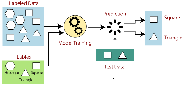
Figure 1: The workflow of supervised machine learning
Terminology and Notation
-
$x$: an input variable/feature
-
$X$: a matrix of multiple features
-
$m$: the total number of training example
-
$n$: the total number of features per one training example
-
$x^{(m)}_{n}$: the value of $n^{th}$ feature in the $m^{th}$ training example
-
$y$: output variable/target variable/label
- $W$: a matrix of weight
-
$f$: function/hypothesis
-
$\hat{y}$: prediction/estimated $y$
-
$b$: a matrix of bias
-
$\alpha$: learning rate
-
$\mu$: sample mean
-
$\sigma$: standard deviation
-
$z$: activation function
-
$L$: loss function
-
$\lambda$: regularization parameter
Cost Function
Cost function, denoted as $J$, is to determine how well the model (or the line or the choice of adjusting $w$ and $b$) fits the training data. The example below is the cost function (i.e. mean squared error - MSE) of linear regression model.
\[\begin{aligned} J(w,b)&= \frac{1}{2m}\sum\limits_{i=1}^{m}{\underbrace{(\hat y^{(i)} - y^{(i)})}_\text{error}}^2 \\ &=\frac{1}{2m}\sum\limits_{i=1}^{m}{( f_{w,b}{(x^{(i)})} - y^{(i)})}^2 \end{aligned}\]where $i$ represents the $i^{th}$ training example, and $b$ and $w$ are training parameters which will be adjusted during the training process.

Figure 2: The error between the predicted value and the actual label
Gradient Descent
Gradient descent algorithm is to minimize the cost function $J$ by finding values of parameters $w$ and $b$. For example, given the cost function $J(W,b)$ and we want to minimize it.
\[\min_{W,b} J(W,b)\]Gradient descent algorithm
-
Step 1: Choose an appropriate $\alpha$ and Randomly initialize $w$ and $b$ parameters
-
Step 2: Repeat until convergence {
\[w=w-\alpha{d \over dw}J(w,b)\]\(b=b-\alpha{d \over db}J(w,b)\) }
Types of gradient descent
-
Batch GD: each training epoch of GD uses all the training example before updating parameters. -
Stochastic GD: each training epoch of GD uses one training example. -
Mini-batch GD: each training epoch of GD uses a small batch size of training example.
Gradient descent tips
-
Feature scaling: is applied to features where their values have a large gap. For example, in the housing price prediciton problem, we have a feature bedrooms $X_1=[x_1, x_2,…,x_n]$ ($1 \le x_1, x_2,…, x_n \le 5$) and a feature size $X_2=[x_1, x_2,…,x_n]$ ($500 \le x_1, x_2,…, x_n \le 1000$).- Mean normalization technique
- Z-score normalization method
If we do not apply feature scaling, features that have larger values than other ones will have a larger impact on the cost function. This is because any small change in the weight value in the former leading to big impact on the value of cost function (these weight values are multiplied with big values of features).
-
Another important question raised is when do we use normalization and standardization
-
Normalization:-
is used when the data doesn’t have Gaussian distribution
-
The value scale falls between [0, 1] or [-1, 1],…
-
-
Standardization:-
is used when the data have Gaussian distribution
-
All features will have a mean $\mu$ of 0 and a standard deviation $\sigma$ of 1.
-
eg: Z-score normalization
-
-
NOTE: It is important to note that we need to normalize/standardize our new data to the same scale as our model works before making a prediction.
Choose a proper learning rate
- Values of $\alpha$ we can try at the firt glance: 0.001, 0.003, 0.01, 0.03, 0.1, 0.3, and so on.
Feature Engineering
It relates to the process of choosing, transforming and combining the most proper features.
Types of supervised learning
-
Regression
- The number of labels is large and the value of the label is a continuous variable, integer,… For example, predicting the housing price,…
-
Classification
- The number of labels is small and the value of the label is a dicrete variable. For example, predicting the given animal is dog or cat,…
We will delve into each of these types in the following.
2. Regression Model
2.1. Linear Regression Model
We fit *a straight line* across data points where *the straight line* is formulated as follows:
\[f_{w,b}(x)=f(x)=\hat y=w{x}+b\]where $W$ and $b$ are parameters learned during the training process. Please refer to terminology here.
Here is the example of using sklearn to implement linear regression. [code link]
2.1. Polynomial Regression Model
We can fit *a curve* across data points. The formula of polynomial regression is denoted as follows:
\[f_{W,b}(X)=f(X)=\hat y=W{X}+b\].png)
Figure 3: Linear regression vs. Polynomial regression
3. Classification Model
3.1. Logistic Regression
Sigmoid function
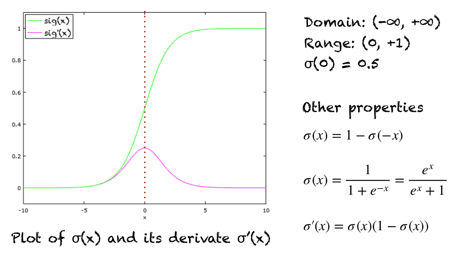
Figure 4: The sigmoid function and its derivative (The axis of x in the figure will be the axis of z for below formulation.)
Formulation
We will consider the logistic regression output $g(z)$ is the probability that class is 1. Particularly, $g(z)$ is the probability that $y$ is 1, given input $X$, parameters $W$ and $b$.
\[z = WX + b\]and
\[\begin{aligned} f_{W,b}{(X)} = \hat y = g(z) &= {1 \over 1 + e ^ {-(WX+b)}} \\ &= {1 \over 1 + e ^ {-z}} \\ &= P(y=1 | X; W, b) \end{aligned}\]where
$f_{W,b}{(X)}$ is the model’s prediction, $g$ is the sigmoid function and $0 \lt g(z) \lt 1$
Decision boundary
It can be a linear/curve decision boundary.

Figure 5: The decision boundary
Cost function for logistic regression
Why don’t we use MSE in logistic regression? Answer: For the case of the linear model, MSE was guaranteed to be convex because it was a linear combination of a prediction function that was also composed. For the case of logistic regression, MSE isn’t guaranteed to be convex because it’s a linear combination between scalars and a function, the logistic function, that’s also not convex.
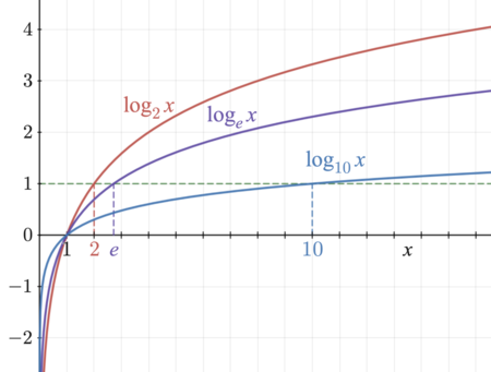
Figure 6: Logarithm functions
To better understand the principles of logistic loss function, we will have a look at how logarithm functions work in the Firgure 6 below.
-
\[\begin{aligned} L(f_{W,b}(x^{(i)}), y^{(i)}) &= \begin{cases} -log(f_{W,b}(x^{(i)})) & \text{if } y^{(i)}=1 \\ -log(1-f_{W,b}(x^{(i)})) & \text{if } y^{(i)}=0 \end{cases} \\ &= -y^{(i)}log(f_{W,b}(x^{(i)}))-(1-y^{(i)})log(1-f_{W,b}(x^{(i)})) \end{aligned}\]Logistic loss function:Therefore, we consider the case of $L(f_{W,b}(X^{(i)}), y)$ when $y^{(i)}=1$ and where $0 \lt f_{W,b}(x^{(i)}) \lt 1$:
-
As $f_{W,b}(x^{(i)}) \to 1$, then $L(f_{W,b}(x^{(i)}), y^{(i)}) \to 0$
-
As $f_{W,b}(x^{(i)}) \to 0$, then $L(f_{W,b}(x^{(i)}), y^{(i)}) \to \infty$
-
NOTE: the term cost function refers to the loss of the entire training set whle the term loss function applies to a single example.
-
\[\begin{aligned} J(W, b)&=\frac{1}{m}\sum\limits_{i=1}^{m}{L(f_{W,b}(x^{(i)}), y^{(i)})} \\ &=-\frac{1}{m}\sum\limits_{i=1}^{m}{[y^{(i)}log(f_{W,b}(x^{(i)}))+(1-y^{(i)})log(1-f_{W,b}(x^{(i)}))]} \end{aligned}\]Logistic cost function:
4. Overfitting
4.1. The problem of overfitting and potential solutions
Definition
Overfitting or high variance happens when a model fits the training data well but does not work well with new examples that are not in the training set.

Figure 7: Examples of overfitting and underfitting in regression and classification problems
Potential solutions
Here are few ways to address overfitting:
-
Collecting more training examples: is to help the model have a bigger picture about the data pool, then it can generalize data effectively.
-
Select most proper features to include/exclude or feature selection: is to help the model works better in terms of metric evaluation and computation.
-
Reduce the size of parameters but keep all features
- Regularization: is to reduce the impacts of some features to the learning model. We will dive into regularization in the below section.
4.2. Regularization
Regularization is to make learning parameters (i.e., mainly $w$) really small or close to $0$ to overcome overfitting.
In practice, it is hard to choose which features we can regularize. Therefore, we will penalize all of them by adding regularization term to the cost function to keep $w_j$ small and fit data.
\[J(w,b)= \frac{1}{2m}\sum\limits_{i=1}^{m}{\underbrace{(f_{W,b}(x^{(i)})- y^{(i)})}_\text{MSE}}^2 + \underbrace{\frac{\lambda}{2m}\sum\limits_{j=1}^{n}{w_j}^2}_\text{regularization term}\]NOTE: Because regularizing $b$ only makes a trivial impact, I only consider regularizing of $w$.
Gradient descent for regularized/logistic linear regression
-
Step 1: Choose an appropriate $\alpha$ and Randomly initialize $w$ and $b$ parameters
-
Step 2: Repeat until convergence {
\[\begin{aligned} w_j&=w_j-\alpha{d \over dw_j}J(w,b) \\ &=w_j - \alpha [\frac{1}{m}\sum\limits_{i=1}^{m}{[(f_{W,b}(x^{(i)})- y^{(i)})(x_{j}^{(i)})]} + \frac{\lambda}{m}w_{j}] \\ &=w_j - \underbrace{\alpha\frac{\lambda}{m}w_{j}}_\text{decrease $w_j$} - \alpha \frac{1}{m}\sum\limits_{i=1}^{m}{(f_{W,b}(x^{(i)})- y^{(i)})(x_{j}^{(i)})} \end{aligned}\]\(b=b-\alpha{d \over db}J(w,b)=b-\alpha[\frac{1}{m}\sum\limits_{i=1}^{m}{(f_{W,b}(x^{(i)})- y^{(i)})}]\) }
You can find the fully-detailed implementation of logistic regression using sigmoid function, cost function, and regularization in the code link.