How Transformer LLMs Work
I have wanted to understand Transformers and related advances in a structured, in-depth way for a long time, but I struggled to find the right resources. I therefore decided to study the topic systematically. These notes synthesize the How Transformer LLMs Work and Attention in Transformers: Concepts and Code in PyTorch courses by DeepLearning.AI with material from other courses and readings I did. I hope they also help others build a clear understanding of Transformers, and I will continue updating them over time.
NOTE: At some points, you and (I) will find it difficult, but believe me, you will find the answer by reading further (I hide it from you and future me in later parts @@).
Table of Contents
- 1. Language Models: Evolution and Fundamentals
- 2. Transformer Architecture
- 3. Processing Pipeline
- 4. Self-Attention
- 5. Mixture of Experts
- 6. References
1. Language Models: Evolution and Fundamentals
1.1. Bag-of-Words
-
We begin with unstructured text.
-
Through tokenization, we divide the text into tokens, such as words.
-
The unique tokens form a vocabulary.
-
A document can then be represented as a numerical vector containing the count or presence of each vocabulary item.
Limitation: Bag-of-Words does not directly represent word order or semantic meaning.
1.2. Static Word Embeddings
Neural methods such as Word2Vec learn dense vector embeddings that capture semantic relationships between words. We can compare these vectors to estimate the similarity between words.
Limitation: Word2Vec creates static embeddings. For example, it produces the same embedding for bank in river bank and financial bank, regardless of the surrounding context.
1.3. RNNs and Attention
-
Recurrent neural networks (RNNs) process a sequence token by token while maintaining a hidden state containing information from previous positions.
-
In an encoder-decoder RNN, the encoder represents the input sequence, and the decoder generates the output sequence autoregressively.
A single fixed-size context vector may fail to preserve all relevant information from a long or complex input sequence.
- Attention allows the decoder to access different encoder states instead of relying on only one context vector. However, the recurrent computation remains sequential, which limits parallelization.
2. Transformer Architecture
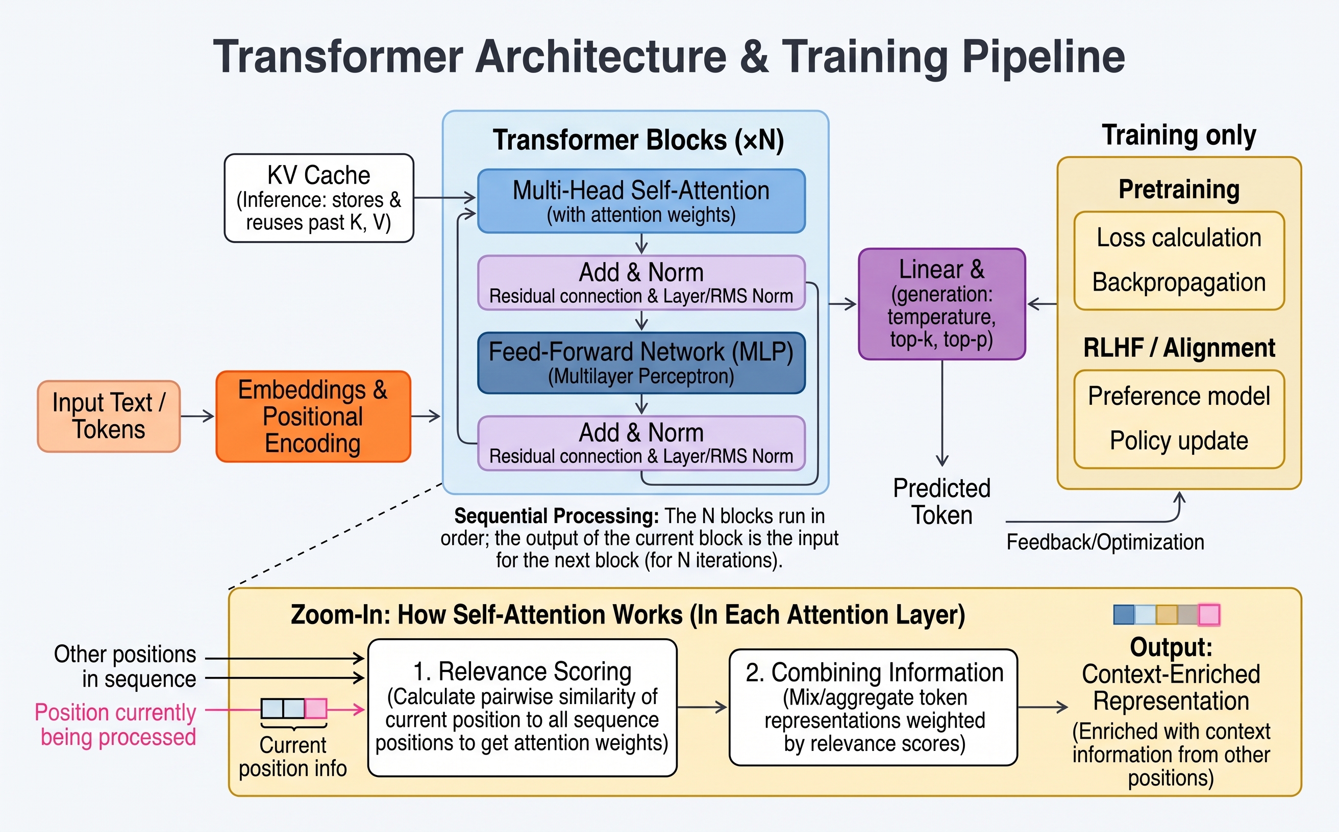
A Transformer consists of a stack of (N) structurally identical layers with separate learned parameters. Each layer uses attention to incorporate/attend information from permitted token positions and a position-wise feed-forward network to transform each token representation independently. The original encoder–decoder Transformer has separate encoder and decoder stacks, with decoder layers additionally using cross-attention over encoder outputs.
2.1. Transformer Encoder
The Transformer encoder converts input token embeddings into contextualized representations using positional information and a stack of encoder layers. Its main components are:
-
Positional information supplies token order. Without it, self-attention with no causal mask is permutation-equivariant: the encoder gives each word in “The dog bit the man” and “The man bit the dog” the same representation, even though who bites whom is reversed. Position can be added to input embeddings or applied within attention:
-
Fixed sinusoidal encodings (additive): the original Transformer adds a non-trainable vector $p_i\in\mathbb{R}^{d_{\text{model}}}$ to the token embedding at position $i$, once, before the first layer 1: $p_{i,2r}=\sin(i\omega_r)$ and $p_{i,2r+1}=\cos(i\omega_r)$, with $\omega_r=10000^{-2r/d_{\text{model}}}$.
Limitations: absolute position is mixed into each token’s content vector once, at the input. Attention does not expose the relative offset between two tokens directly, so the model must learn it from this mixture, and deeper layers receive position only through the residual stream. RoPE instead injects relative position into every attention layer (see Section 4.1 for the formulation).
-
Rotary position embeddings (RoPE): every attention layer rotates each 2-D pair of query and key dimensions by an angle proportional to the token’s position; the embeddings themselves are unchanged. The query-key dot product then depends on position only through the relative offset between the two tokens 2.
-
-
Multi-head self-attention: multiple heads can use different learned projections for queries, keys, and values from the same input token representations (see Section 4.3.5). This lets each token gather different kinds of context from other tokens in the input sequence.
-
Layer Norm 3: normalizes the features of each token representation separately, helping stabilize training. Its placement within a Transformer block depends on the architecture.
-
Position-wise feed-forward network (Position-wise FFN): applies the same nonlinear transformation to each contextualized token representation independently.
2.2. Transformer Decoder
In the original encoder-decoder Transformer, the decoder generates the output sequence using previously available output tokens and the encoder’s contextualized input representations. Each decoder layer contains:
-
Masked self-attention: applies a causal mask so that each position can attend only to itself and earlier positions.
-
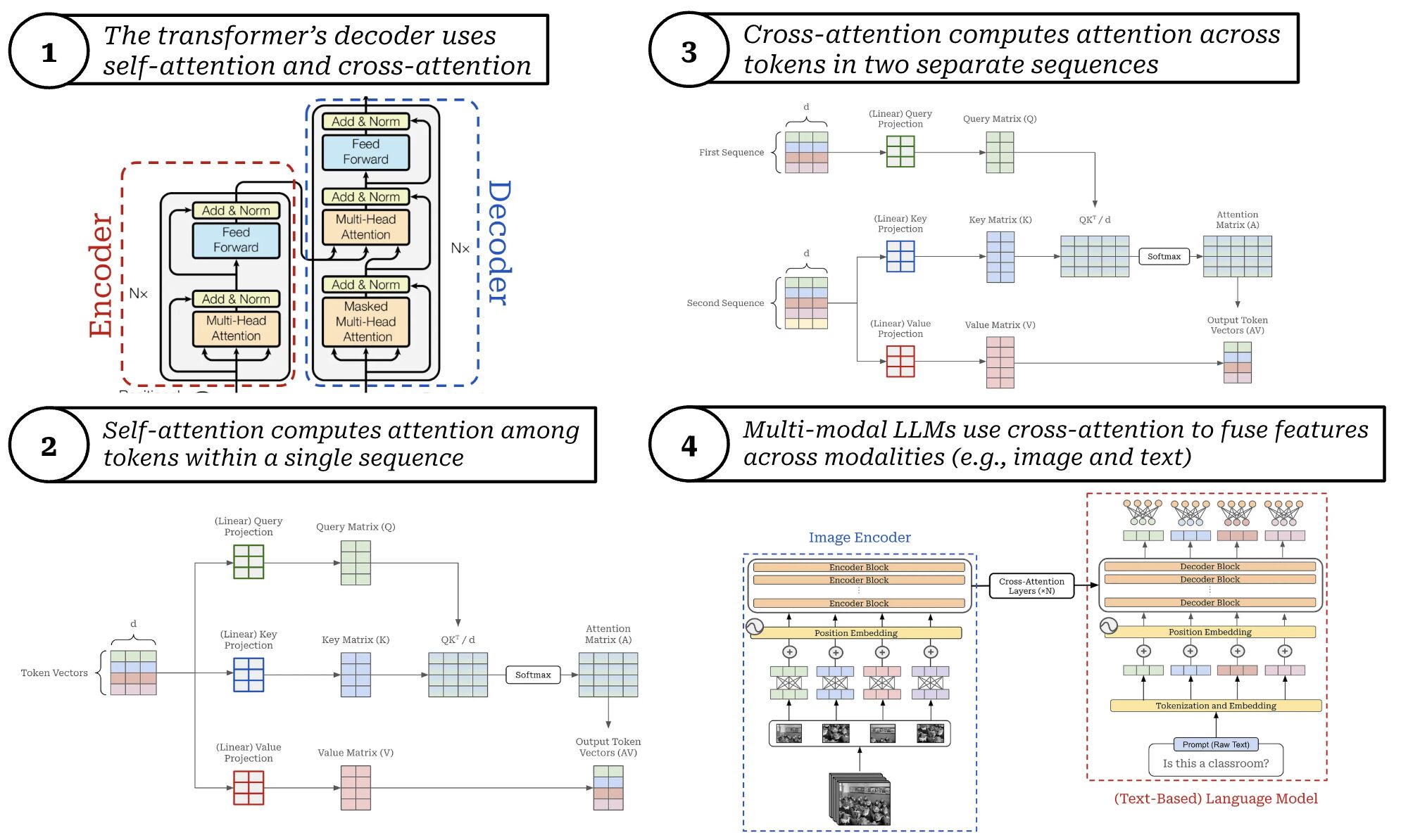
Encoder-decoder attention or Cross-attention (in traditional encoder-decoder transformer): uses decoder representations (i.e., output of the masked self-attention described in Section 4.2) as queries and encoder outputs as keys and values. You can look at the sub-figure 4 below, where we have an example for using cross attention for multimodal.
Later, researchers have found out that using encoder-only and decoder-only can work well for different applications.
- Position-wise feed-forward network: applies a nonlinear transformation to each token representation independently.
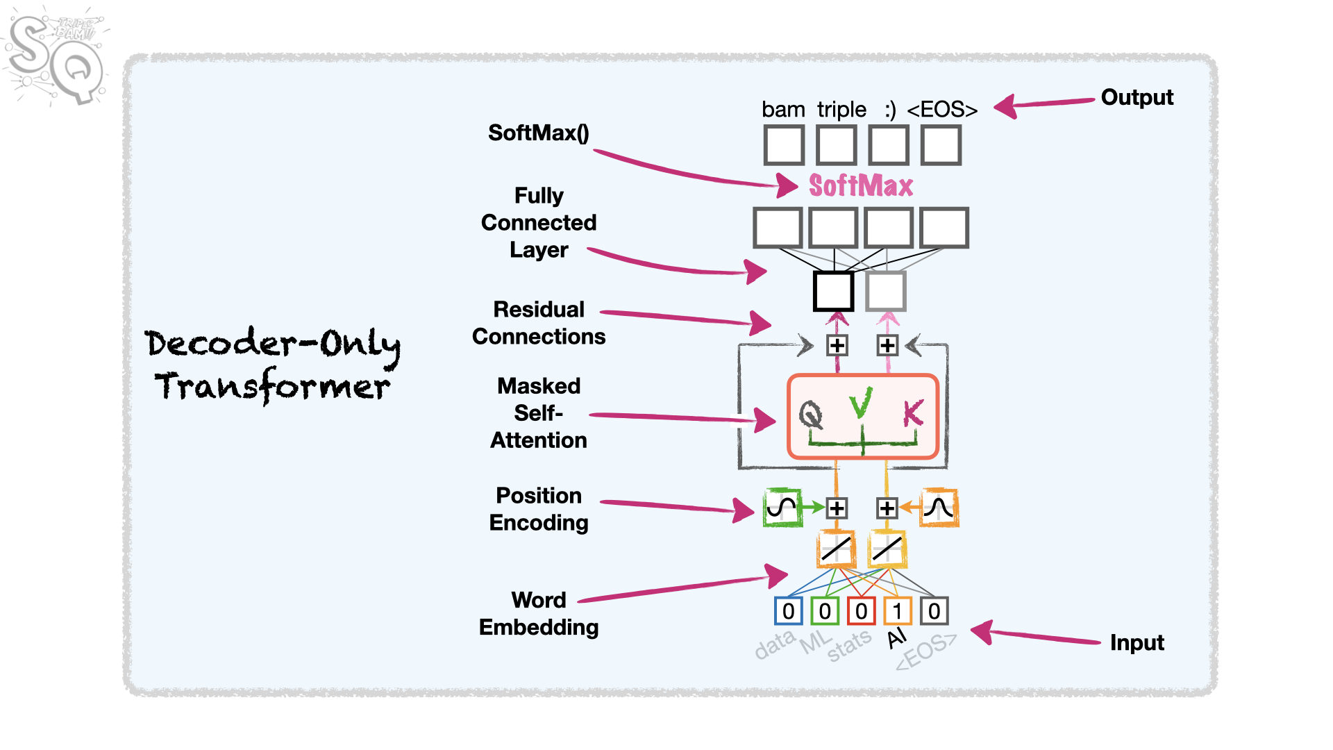
A final linear layer and softmax convert a decoder hidden state into a probability distribution over the vocabulary.
To avoid confusion among concepts of attention, we can remember them as follows: Bidirectional self-attention allows each token to attend to all unmasked tokens (e.g., BERT), masked/causal self-attention blocks each token to attend to future tokens (e.g., GPT), encoder-decoder attention/cross-attention lets decoder representations (i.e., queries) to attend to encoder outputs (keys and values) (e.g., multimodal).
2.3. Encoder-Only and Decoder-Only Transformers
-
Encoder-only models, such as BERT, produce contextualized representations for all input tokens. During masked-language-model pre-training, BERT masks selected input tokens and learns to predict their original values. It can then be fine-tuned for downstream tasks.
-
BERT uses bidirectional self-attention, so each ordinary token can attend to tokens on both sides.
-
The final representation of
[CLS]is commonly used for sequence-level tasks after suitable training.[SEP]marks the end of a sequence or separates a pair of sequences. -
Training strategy (BERT) [^10]4:
-
Step 1 (Self-supervised pre-training): Learn general language representations from large amounts of unlabeled text using proxy tasks, with targets derived automatically from the text. This is usually the most computationally expensive stage.
-
Masked Language Modeling (MLM): select 15% of input tokens for prediction. Of those selected, replace 80% with
[MASK], 10% with a random token, and leave 10% unchanged. Predict the original tokens using context from both sides, and compute the MLM loss only at selected positions. -
Next Sentence Prediction (NSP): use the
[CLS]representation to classify whether text segment B follows segment A in the source document. Half the training pairs are consecutive; half pair A with a random segment from another document. -
Optimize MLM and NSP jointly, using the sum of their losses.
-
-
Step 2: Supervised fine-tuning. Add a task-specific output head and train it together with the pre-trained encoder on labeled data, e.g., for sentiment classification or named entity recognition. This usually requires much less data and computation than pre-training.
-
Scope: this recipe describes the original BERT. NSP is optional in encoder-only training. RoBERTa, for example, uses MLM without NSP 5.
-
-
-
Decoder-only models, such as GPT, use causal self-attention and learn to predict the next token from the preceding tokens.
- Each position can attend only to itself and earlier positions. This causal attention mask differs from BERT’s token masking: GPT hides future attention connections, whereas BERT replaces selected input tokens and predicts them using context from both sides.
2.4. Context Length
The context length is the maximum number of tokens that a model can process in one forward pass. During generation, the context contains the prompt and previously generated tokens.
3. Processing Pipeline
3.1. Tokenization
A tokenizer divides the input into tokens and maps each token to a discrete token ID. Tokenizers may operate at the word, subword, character, or byte level. Subword tokenization is widely used.
Text:      "Transformers are useful"
Tokens:    ["Transform", "ers", "are", "useful"]
Token IDs: [5812, 1047, 389, 7421]
Each tokenizer has a fixed vocabulary size of $v_{\text{tab}}$, which determines how many distinct tokens it can represent.
A larger vocabulary can represent common words or phrases using fewer tokens. However, it also increases the size of the embedding table and, in a language model, the vocabulary-output layer.
3.2. Embeddings
After tokenization, the model uses each token ID to look up a learned vector, called a token embedding, in an embedding table of shape $v_{\text{tab}} \times d_{\text{model}}$, where $v_{\text{tab}}$ is the vocabulary size. For a sequence of $n$ tokens, the lookup produces a matrix of token embeddings in $\mathbb{R}^{n \times d_{\text{model}}}$. Each row is one token’s embedding, and each column is one embedding feature across the tokens.
The transformer also needs positional information to distinguish token order. In models that use additive positional information, the model adds one position vector to each token embedding. For $n$ tokens, the position vectors form a matrix in $\mathbb{R}^{n \times d_{\text{model}}}$, so the resulting input embeddings have the same shape. Other models, such as those using RoPE, apply positional information within the attention mechanism.
Token embeddings are learned during training. Position vectors can be learned too, or they can be fixed. For example, the original Transformer in Attention Is All You Need used fixed positional encodings: sine and cosine functions produce a vector for each position, which is added to the token embedding and does not change during training.
3.3. Transformer Processing
Transformer layers convert the input embeddings into contextualized token representations.
-
An encoder-only model can use these representations for tasks such as classification, retrieval, and token labeling.
-
A decoder-only language model passes its contextualized representations through an LM head to produce next-token probability distributions. During generation, it uses the distribution at the final position to select the next token.
3.4. Layer Norm
-
Layer normalization (LayerNorm) uses the mean and variance across the features of each token representation to normalize that token’s vector. Updates to model parameters such as the embedding table and attention and FFN weights can change the scale of token representations. LayerNorm reduces these shifts, giving the following operations more consistently scaled inputs and making optimization more stable. Its placement depends on the architecture.
-
In a pre-norm block such as nanoGPT, LayerNorm is applied before self-attention and again before the feed-forward network (FFN). nanoGPT also applies a final LayerNorm once after all Transformer blocks.
-
In the original post-norm Transformer shown in the architecture diagram, each Add & Norm box means: add a sublayer’s input to its output (a residual connection), then apply LayerNorm to the sum. The encoder has an Add & Norm after self-attention and another after the FFN. The decoder has three: one after masked self-attention, one after cross-attention, and one after the FFN. The top Add & Norm in the diagram is therefore a normalization after the FFN inside each decoder layer.
-
-
LayerNorm operation: For each token representation $x$, calculate the mean $\mu_x$ and variance $\sigma_x^2$ across its features, then compute $\operatorname{LayerNorm}(x)=\gamma\odot\frac{x-\mu_x}{\sqrt{\sigma_x^2+\epsilon}}+\beta$. Here $\gamma$ and $\beta$ are LayerNorm’s own trainable scale and shift parameters; they act on the normalized vector. The earlier weight updates refer to parameters that produce $x$, such as the embedding, attention, and FFN weights. In a pre-norm block, the result is passed to the attention or FFN.
4. Self-Attention
Self-attention updates each token representation (one row of the input matrix $X$) by combining information from other permitted positions in the same sequence. Which positions are permitted depends on the attention mask: bidirectional models (e.g., BERT) can usually use both earlier and later tokens, while causal models (e.g., GPT) cannot use/attend future tokens.
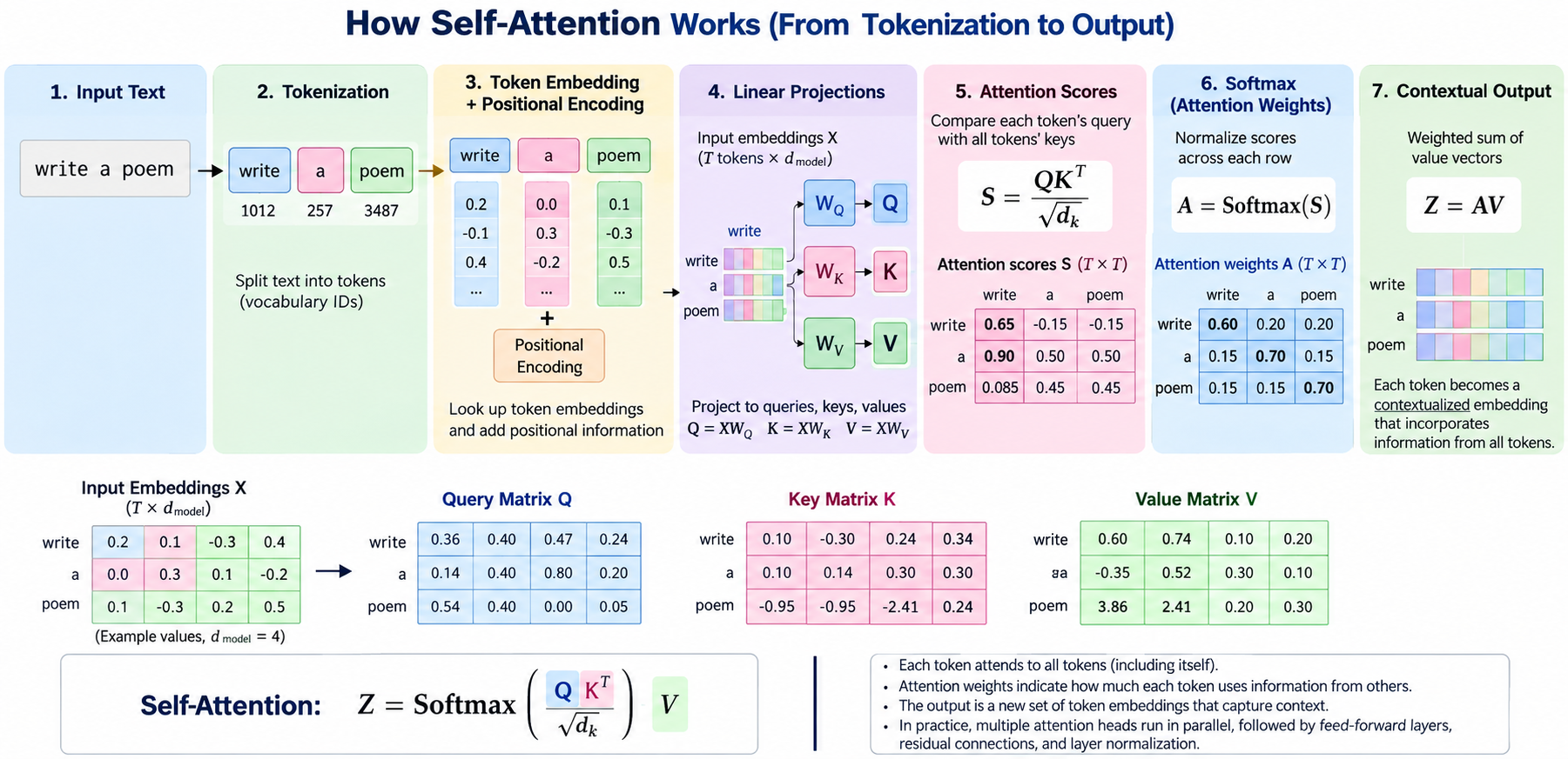
The diagram shows additive positional information and unrestricted attention for simplicity. Some architectures instead apply position information to $Q$ and $K$; for example, RoPE rotates them before their dot products are calculated. You can find an example for single-head (masked) self-attention class below:
class MaskedSelfAttention(nn.Module):
    def __init__(self, d_model=2, # dimension for each input token embedding
                 row_dim=0, # row and column indexes
                 col_dim=1):

        super().__init__()

        self.W_q = nn.Linear(in_features=d_model, out_features=d_model, bias=False)
        self.W_k = nn.Linear(in_features=d_model, out_features=d_model, bias=False)
        self.W_v = nn.Linear(in_features=d_model, out_features=d_model, bias=False)

        self.row_dim = row_dim
        self.col_dim = col_dim

    # This method is to calculate the (masked) self-attention values for each token
    def forward(self, token_encodings, mask=None):

        q = self.W_q(token_encodings)
        k = self.W_k(token_encodings)
        v = self.W_v(token_encodings)

        sims = torch.matmul(q, k.transpose(dim0=self.row_dim, dim1=self.col_dim))

        scaled_sims = sims / torch.tensor(k.size(self.col_dim)**0.5)

        if mask is not None:
            ## Here we are masking out things we don't want to pay attention to
            ##
            ## We replace values we wanted masked out
            ## with a very small negative number so that the SoftMax() function
            ## will give all masked elements an output value (or "probability") of 0.
            scaled_sims = scaled_sims.masked_fill(mask=mask, value=-1e9) # I've also seen -1e20 and -9e15 used in masking

        attention_percents = F.softmax(scaled_sims, dim=self.col_dim)

        attention_scores = torch.matmul(attention_percents, v)

        return attention_scores
4.1. From Hidden States to $Q$, $K$, and $V$
In self-attention, $X \in \mathbb{R}^{N \times d_{\text{model}}}$ contains one token representation per sequence position, where $N$ is the sequence length and $d_{\text{model}}$ is the representation size. In the first Transformer block, $X$ is derived from token embeddings plus any positional vectors added at the input. In later blocks, it is derived from the preceding block’s representations. In a pre-norm block, $X$ is the LayerNorm output of those representations. Thus, $Q$, $K$, and $V$ are projections of the representations entering the current self-attention layer. Methods such as RoPE apply positional information to $Q$ and $K$ after the projections. In standard multi-head attention with $h$ heads, each head usually has $d_k=d_{\text{model}}/h$ query and key dimensions. See 3 for a visualization.
For each token in one attention head, three learned linear projections produce6:
\[Q = XW^Q, \qquad K = XW^K, \qquad V = XW^V\]where $W^Q,W^K \in \mathbb{R}^{d_{\text{model}} \times d_k}$ and $W^V \in \mathbb{R}^{d_{\text{model}} \times d_v}$. Therefore, $Q,K \in \mathbb{R}^{N \times d_k}$ and $V \in \mathbb{R}^{N \times d_v}$.
| The question it answers | Its role | |
|---|---|---|
| Query $Q$ | “What am I looking for?” | The token doing the looking |
| Key $K$ | “What am I?” | How a token advertises itself |
| Value $V$ | “What do I contribute if chosen?” | The content actually retrieved |
Separate projections let the model learn different representations for matching and for transferring information. In particular, $QK^T$ can express directional relationships, whereas $XX^T$ is symmetric.
Training note: When training from scratch, the token embeddings and projection matrices normally begin with random values and are updated by backpropagation. Learned positional embeddings are updated too; fixed positional encodings are not. By contrast, $X$, $Q$, $K$, and $V$ are temporary activations. They are recomputed on every forward pass and change as the model parameters change.
Additive positions in the attention score: in the first block of the original (post-norm) Transformer, row $i$ of $X$ is $x_i=e_i+p_i$. The query at position $i$ is then $q_i=x_iW^Q$ (row $i$ of $Q$), the key at position $j$ is $k_j=x_jW^K$ (row $j$ of $K$), and the raw score $(QK^T)_{ij}=q_ik_j^T$ splits into content-content, content-position, position-content, and position-position terms:
\[q_ik_j^T=e_iW^Q{W^K}^Te_j^T+e_iW^Q{W^K}^Tp_j^T+p_iW^Q{W^K}^Te_j^T+p_iW^Q{W^K}^Tp_j^T.\]The second and third terms are cross terms: each pairs one token’s content with the other token’s absolute position ($p_j$ or $p_i$), not with the offset $j-i$. Without projection, the sinusoidal encodings from Section 2.1 satisfy $p_ip_j^T=\sum_r\cos\big((j-i)\omega_r\big)$, a function of the offset $j-i$ alone, but the learned $W^Q{W^K}^T$ generally breaks this. RoPE avoids the problem by rotating $q_i$ and $k_j$ so that their dot product depends on position only through $j-i$ (see Section 4.3.5).
Example: suppose the model should learn the rule “attend to the previous token”, i.e., the offset $j-i=-1$ for query-key pairs such as $(3,2)$, $(7,6)$, and $(100,99)$.
- Additive: each pair uses different position vectors ($p_3,p_2$ vs. $p_7,p_6$ vs. $p_{100},p_{99}$), so the scores differ even for identical words. The model must learn from training data at many positions that these pairs mean the same thing.
- RoPE: every pair uses the same rotation $R_{-1}$, so identical words give identical scores. A rule learned at one position holds at every position.
4.2. Scaled Dot-Product Attention
One attention head computes 7:
\[S = \frac{QK^T}{\sqrt{d_k}} + M, \qquad A = \operatorname{softmax}(S), \qquad Z = AV\]-
Score: $QK^T$ compares every query with every key, answering the question: How relevant is each key token to this query token? Dividing by $\sqrt{d_k}$ keeps large dot products from saturating the softmax function.
- Why divide by $\sqrt{d_k}$ 6? Answer: Each raw attention logit is a dot product containing $d_k$ terms. Under the simplifying assumptions that the query and key components are independent, zero-centered, and have unit variance, the logit has variance $d_k$ and standard deviation $\sqrt{d_k}$. Without scaling, wider heads therefore produce larger gaps between logits, which can make the softmax overly concentrated and its gradients very small. Dividing by $\sqrt{d_k}$ approximately normalizes the logit variance to $1$, keeping the softmax scale and gradients more consistent across head dimensions. This does not make different heads or head counts equivalent; it only removes the unintended growth in score magnitude, while each head can still learn distinct attention patterns.
-
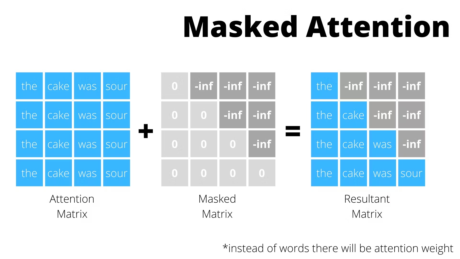
Mask: $M$ is $0$ for allowed query-key pairs and $-\infty$ (or a very large negative value) for blocked pairs. In causal self-attention, it blocks access to future tokens; after softmax, blocked positions receive zero or effectively zero attention weight. A causal mask is unnecessary in bidirectional self-attention, although a padding mask may still be used. For example:
-
Normalize: Apply softmax to each row of the scaled, masked score matrix $S$. For query position $i$, $A_{ij}=e^{S_{ij}}/\sum_k e^{S_{ik}}$ gives the weight assigned to key position $j$. The weights in each row are nonnegative and sum to $1$, and they determine how much each corresponding value vector contributes to that query’s output.
-
Combine: $AV$ produces $Z$, a weighted sum of value vectors for each query position/token. For each token, relevant tokens get large weights, giving each token its answer 6.
For self-attention over $N$ tokens, $S,A \in \mathbb{R}^{N \times N}$ and $Z \in \mathbb{R}^{N \times d_v}$.
A dot product depends on both vector direction and magnitude. Unlike cosine similarity, it is not normalized to the range $[-1,1]$.
4.3. Multi-Head Attention and Efficient Variants
Transformers run several attention heads in parallel. Each head produces an output $Z$ as described in Section 4.2 and can learn different relationships.
4.3.1. Projection
For each token, the head outputs are concatenated along the feature dimension, then mixed by the output projection $W^O$:
\[\operatorname{MultiHead}(X) = \operatorname{Concat}(\text{head}_1, \ldots, \text{head}_h)W^O.\]4.3.2. Residual Connections
We now have the output of the multi-head self-attention sublayer. We add it element-wise to the sublayer’s input, i.e., the token representations entering the layer (for the first layer, these are the input embeddings). This is called a residual (skip) connection. It is also why $W^O$ projects the concatenated heads back to $d_{\text{model}}$: both terms of the sum must have the same shape.
- Pre-norm (e.g., GPT-2, nanoGPT): $x’ = x + \operatorname{MultiHead}(\operatorname{LayerNorm}(x))$.
- Post-norm (original Transformer, Add & Norm): $x’ = \operatorname{LayerNorm}(x + \operatorname{MultiHead}(x))$.
Why do we need residual connections 8?
Gradient flow (backward pass): by the chain rule, the gradient reaching an early layer is a product of the Jacobians of all later layers (weight matrices, activation derivatives, normalization, softmax). If many of these factors shrink the gradient, their product can become very small (vanishing gradients). With a residual connection $y = x + F(x)$, the Jacobian (e..g, which is a set of derivatives using for vectors) becomes $\frac{\partial y}{\partial x} = I + \frac{\partial F}{\partial x}$, so $\frac{\partial \mathcal{L}}{\partial x} = \frac{\partial \mathcal{L}}{\partial y} + \frac{\partial \mathcal{L}}{\partial y}\frac{\partial F}{\partial x}$. The identity term passes the gradient back unchanged, even when $\frac{\partial F}{\partial x}$ is small. Stacking blocks gives $x_L = x_l + \sum_{i=l}^{L-1} F_i(x_i)$, so every earlier layer, including the embedding table, receives a direct gradient signal from the output 9.
Preserving token information (forward pass): within each head, $AV$ makes every token’s output a weighted average of the value vectors of the tokens it attends to. This lets tokens share context, but it also dilutes each token’s own information and pulls token representations toward each other. Concatenating the heads and applying $W^O$ cannot undo this, because they only mix features within each token’s concatenated head outputs, not across tokens. So when many attention layers are applied one after another without residual connections, token representations become increasingly similar. The residual connection keeps each token’s own representation in the sum, so each layer adds context instead of overwriting it 10.
Note: the clean identity path above holds for pre-norm blocks. In post-norm blocks, LayerNorm sits on the residual path after every addition, so the gradient must also pass through each LayerNorm; deep post-norm Transformers are harder to train and usually rely on learning-rate warm-up 11.
4.3.3. Feed-Forward Network (FFN)
Let $h$ be the output of the attention sublayer after its residual connection. The position-wise FFN (Section 2.1) is a small multi-layer perceptron (MLP): a linear layer expands each token’s vector (typically to $4\,d_{\text{model}}$), a nonlinear activation $\phi$ is applied, and a second linear layer projects it back to $d_{\text{model}}$:
\[\operatorname{FFN}(x) = \phi(xW_1 + b_1)\,W_2 + b_2.\]The original Transformer uses ReLU for $\phi$; BERT and GPT-2 use GELU; many recent LLMs, such as Llama, use a gated variant (SwiGLU). The FFN is wrapped with LayerNorm and a residual connection in the same way as attention (Section 4.3.2), which gives the output of the Transformer block, i.e., the input to the next block:
- Pre-norm: $\text{out} = h + \operatorname{FFN}(\operatorname{LayerNorm}(h))$.
- Post-norm: $\text{out} = \operatorname{LayerNorm}(h + \operatorname{FFN}(h))$.
Normalization evolution: Nowadays, Pre-norm and RMSNorm are widely used.
4.3.4. Output
In a decoder-only LLM, only the output of the last Transformer block, $H \in \mathbb{R}^{n \times d_{\text{model}}}$ (one row $h_i$ per position), is converted into next-token predictions. A pre-norm model first applies a final LayerNorm (Section 3.4). The LM head, a single linear layer (not an MLP), then maps each row to $v_{\text{tab}}$ scores called logits, one per vocabulary token:
\[\text{logits} = H\,W_{\text{LM}} \in \mathbb{R}^{n \times v_{\text{tab}}}, \qquad W_{\text{LM}} \in \mathbb{R}^{d_{\text{model}} \times v_{\text{tab}}}.\]Many models, such as GPT-2, reuse the token embedding table $E \in \mathbb{R}^{v_{\text{tab}} \times d_{\text{model}}}$ (Section 3.2) as this matrix, i.e., $W_{\text{LM}} = E^T$ (weight tying). The logit of token $k$ at position $i$ is then simply the dot product $h_i \cdot e_k$ between the hidden state and token $k$’s embedding, so a token scores high when the hidden state is aligned with its embedding. Other models, such as Llama 3 8B, learn a separate $W_{\text{LM}}$ of the same shape.
Softmax is applied to each position’s logits separately, giving $n$ probability distributions over the vocabulary. The distribution at position $i$ predicts token $i+1$: training uses all $n$ of them, while generation uses only the last one (Section 3.3).
Example (weight tying, $v_{\text{tab}} = 4$, $d_{\text{model}} = 2$): for the input “the cat”, suppose the final hidden state at the last position is $h_2 = [1, 2]$. Each logit is the dot product of $h_2$ with one row of $E$:
| Token $k$ | the | cat | sat | mat |
|---|---|---|---|---|
| Embedding $e_k$ (row of $E$) | $[1, 0]$ | $[0, 1]$ | $[1, 1]$ | $[-1, 0]$ |
| Logit $h_2 \cdot e_k$ | $1$ | $2$ | $\mathbf{3}$ | $-1$ |
| Probability (softmax) | $0.09$ | $0.24$ | $\mathbf{0.66}$ | $0.01$ |
The model therefore predicts sat as the next token. Computing all four dot products at once is exactly the matrix product $h_2 E^T$.
4.3.5. Variants
-
Multi-head attention (MHA): gives each head its own query, key, and value projections.
-
Motivation: a single attention head produces only one attention distribution for each query token. If several relationships are relevant at the same time, that head may have to combine them into one distribution. Multiple heads can instead learn complementary attention patterns. For example, one head may focus on a token’s referent while another captures a descriptive or syntactic relationship.
-
As a simplified illustration, consider it in the sentence “The trophy didn’t fit in the suitcase because it was too big”:
trophy suitcase big Hypothetical reference score 4 0 0 Hypothetical descriptive score 0 0 4 One combined distribution 0.50 0.01 0.50 Reference-focused head 0.96 0.02 0.02 Description-focused head 0.02 0.02 0.96
-
-
MHA therefore applies attention several times in parallel using different learned projections of the same input representations. The resulting head outputs are concatenated and mixed, allowing each token to gather complementary contextual information from other tokens.
Causal-attention note: in a decoder-only LLM, it cannot attend to the later word big. The example above applies directly to bidirectional attention; in causal attention, a later token can still attend to both it and trophy.
-
-
Multi-query attention (MQA): lets all query heads share one key head and one value head, reducing the key-value cache and memory bandwidth during generation.
-
Grouped-query attention (GQA): lets groups of query heads share key and value heads, providing a compromise between MHA and MQA.
-
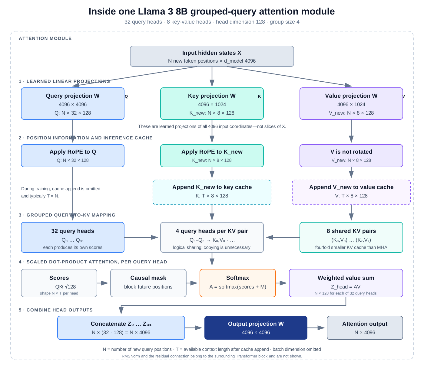
Llama 3 8B example: the model has $d_{\text{model}}=4096$, $32$ query heads, and $8$ key-value heads. Each head has dimension $d_{\text{head}}=4096/32=128$, so each key-value head is shared by a group of $32/8=4$ query heads.
-
Step 1—project: for a sequence representation $X\in\mathbb{R}^{N\times4096}$, the learned projections produce
\[Q=XW^Q\in\mathbb{R}^{N\times4096},\qquad K=XW^K\in\mathbb{R}^{N\times1024},\qquad V=XW^V\in\mathbb{R}^{N\times1024},\]where $W^Q\in\mathbb{R}^{4096\times4096}$ and $W^K,W^V\in\mathbb{R}^{4096\times1024}$. Thus, unlike standard MHA, Llama 3 8B does not produce 4096-dimensional $K$ and $V$ tensors. See Section 4.1 for more about these projection matrices.
-
Step 2—reshape into heads: $Q$ is reshaped into $32$ query heads of width $128$, whereas $K$ and $V$ are each reshaped into $8$ heads of width $128$. These are slices of the projected tensors, not slices of the original input. Because the projection matrices are dense, every head can learn from all $4096$ coordinates of each input token representation.
-
Step 3—share key-value heads: each group of four query heads uses the same key and value head. Every query head still computes its own attention distribution over the allowed token positions, but the four heads in a group attend using shared keys and retrieve information from shared values.
-
Step 4—combine the outputs: the $32$ query-head outputs, each of width $128$, are concatenated into a $4096$-dimensional representation. The output projection $W^O\in\mathbb{R}^{4096\times4096}$ then mixes information across the heads. Using only $8$ key-value heads instead of $32$ reduces the attention key-value cache by a factor of four relative to MHA with the same head dimensions.
-
-
Staying with Llama 3 8B, we can look at other components with concepts and workflows we have seen so far:
-
Token embeddings: the vocabulary size is $128256$, each token is represented by $4096$ numbers.
-
RoPE: Rotary position embeddings apply position-dependent rotations to the query and key vectors before computing their dot product. For a query $q_i$ (row $i$ of $Q$) and a key $k_j$ (row $j$ of $K$), with $R_i$ the rotation for position $i$,
\[q_i'=q_iR_i^T,\qquad k_j'=k_jR_j^T,\qquad q_i'{k_j'}^T=q_iR_i^TR_jk_j^T=q_iR_{j-i}k_j^T.\]Thus, position affects the attention score through the relative offset $j-i$. For example, token pairs at positions $(5,4)$ and $(9,8)$ have different absolute positions but the same offset $-1$, so identical content produces the same positional relationship under RoPE. Additive encodings, by contrast, leave the model to learn this relationship through its projections (see Section 4.1). RoPE is not applied to $V$ because values carry the content retrieved after the attention weights are determined.
-
-
-
Sparse attention: restricts each query to selected positions, reducing the cost of long sequences.
-
Ring Attention: distributes long-sequence attention across devices by circulating blocks of keys and values.
5. Mixture of Experts
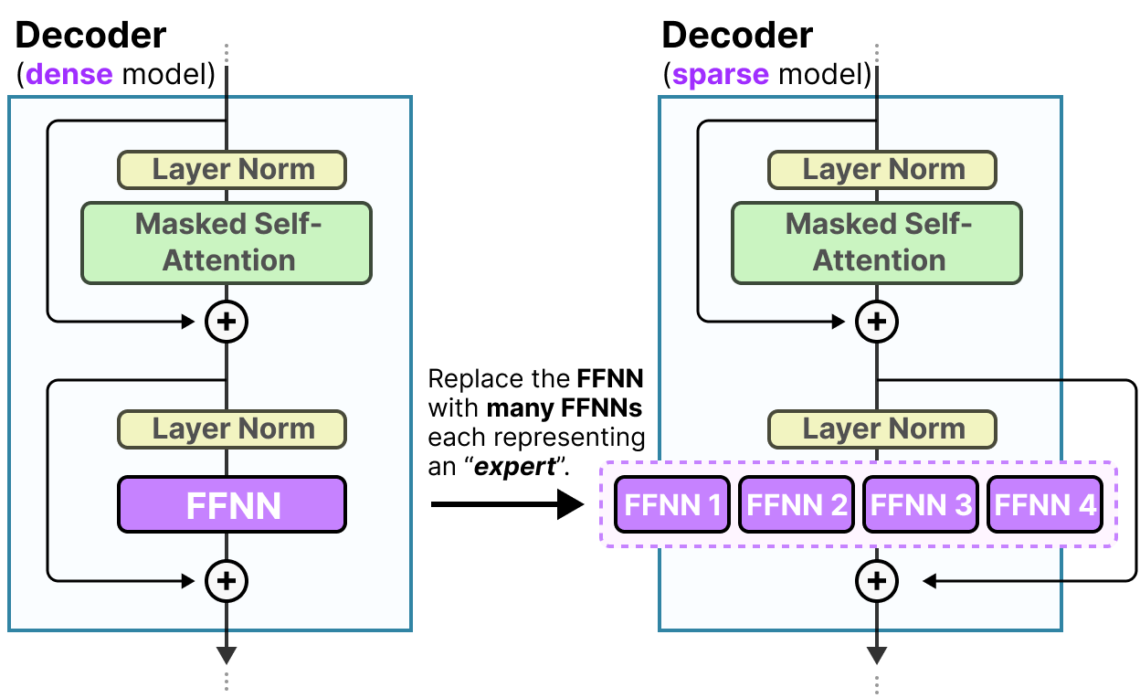
Mixture of Experts (MoE) 12 increases a model’s parameter capacity without activating all parameters for every token. In selected Transformer layers, MoE replaces the traditional FFN with multiple FFNs, called experts.
5.1. Experts and Routers
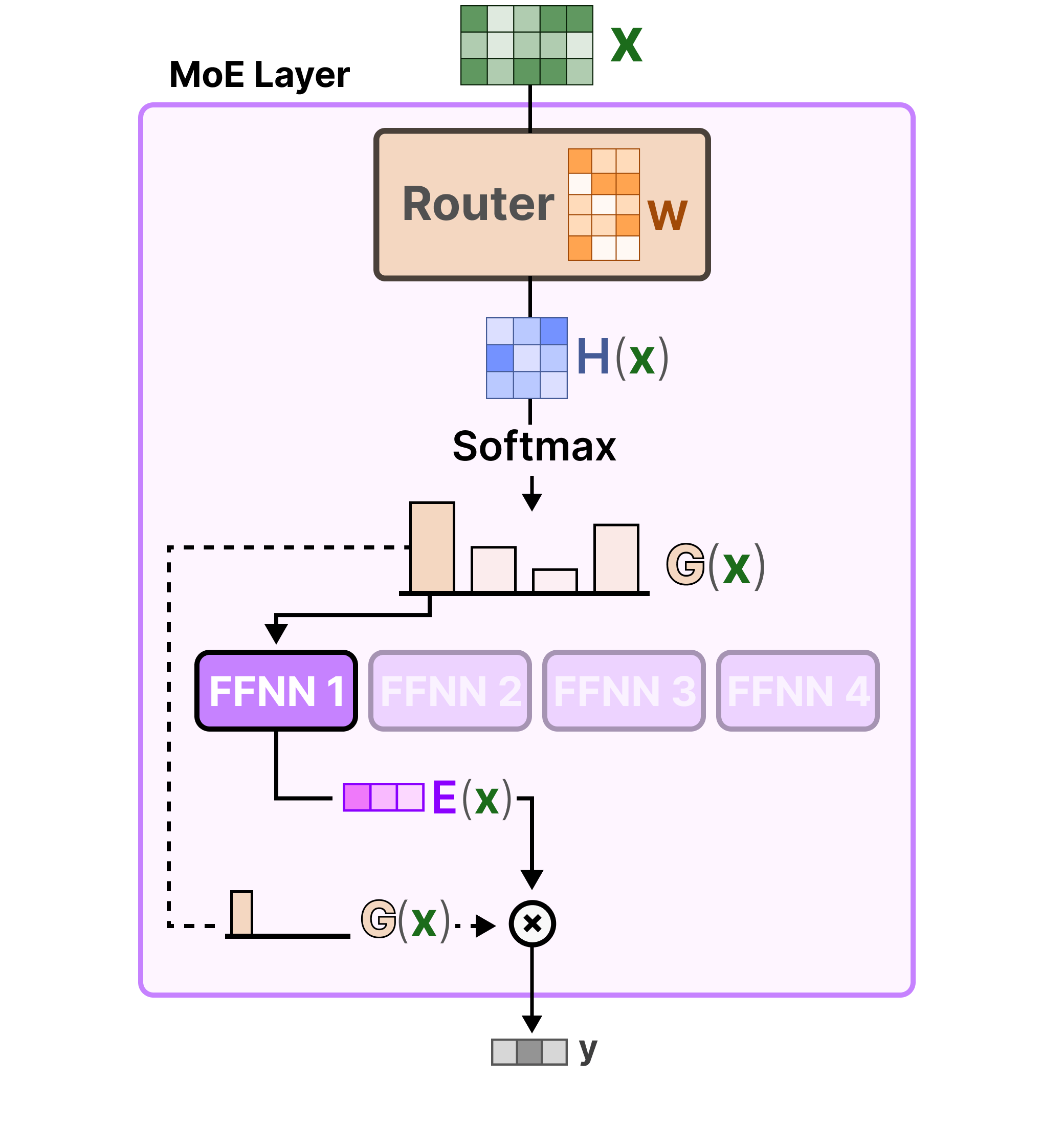
- Intuition: each MoE layer has a set of experts. A router selects a small subset of them to process each token representation. Different experts may learn different patterns, although their specializations are not always easy to interpret.
-
Expert: is normally an FFN within an MoE layer.
-
Gate/Router: is a small learned gating function, often a linear layer, that assigns each expert a score for a given token representation. It selects, for example, the top-$k$ highest-scoring experts and combines their outputs.
-
Routing collapse: the router may learn to favor a few experts early in training. These experts receive more tokens and training updates, which can reinforce the preference while leaving other experts under-trained.
-
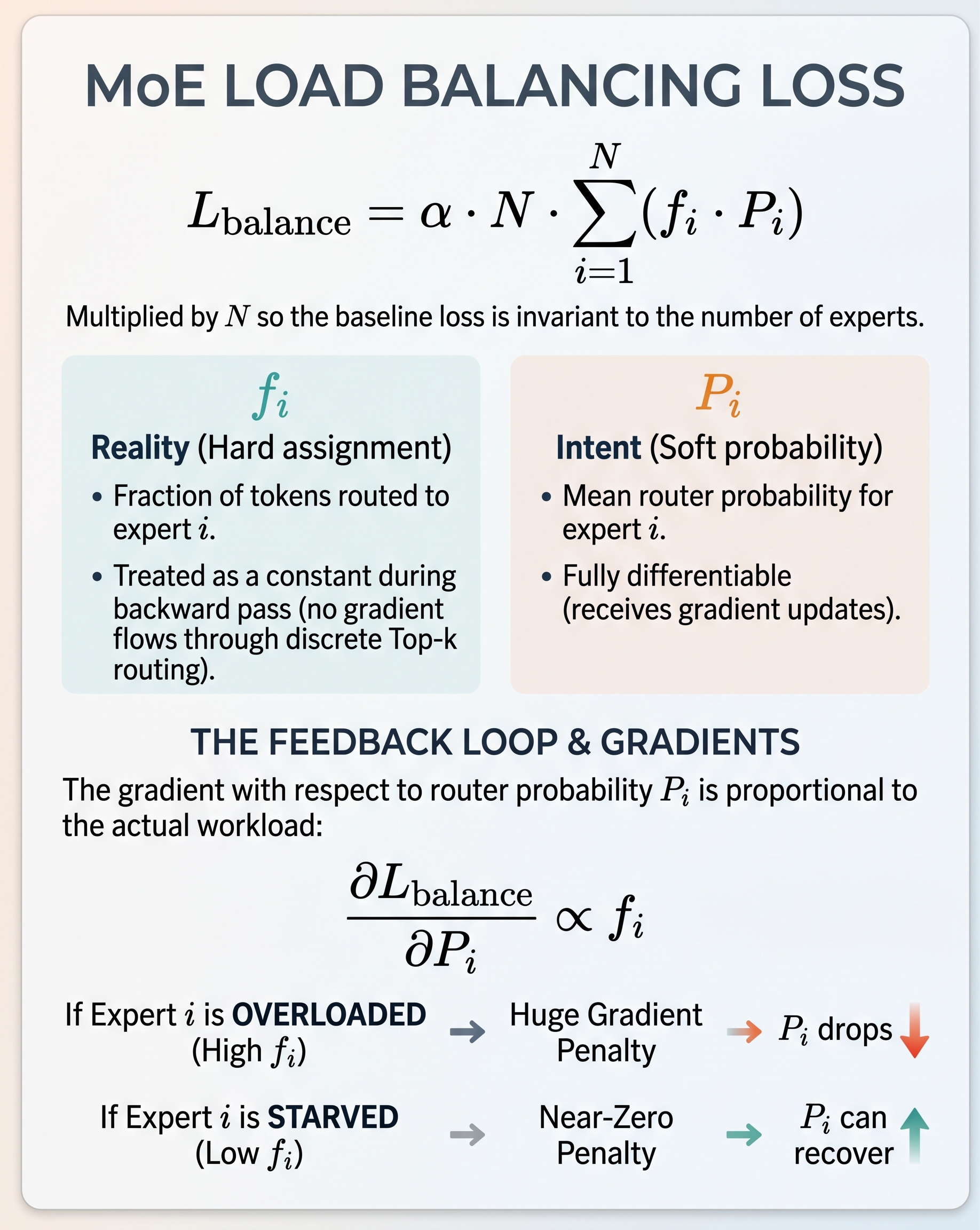
Remedy: add an auxiliary load-balancing loss to the main training loss to encourage more balanced expert usage. For example, Switch Transformer uses the following loss for top-1 routing 13:
\[\mathcal{L}_{\mathrm{balance}}=\alpha E\sum_{i=1}^{E} f_i P_i,\]where $E$ is the number of experts, $f_i$ is the fraction of tokens in a batch assigned to expert $i$, $P_i$ is the router’s probability for expert $i$ averaged over all tokens in that batch, and $\alpha$ controls the loss strength. Gradients flow through $P_i$, while the discrete assignment fractions $f_i$ are treated as constants. This pushes probability away from heavily used experts. You can see the illustrated image below.
-
5.2. Total and Active Parameters
-
Total parameters include the input embeddings, attention layers, routers, all experts, and the LM head. During standard inference, all experts must be available in memory, although they may be distributed across multiple devices.
-
Active parameters are the parameters used to process a particular token. Only the selected top-$k$ experts are activated for that token. This is why MoE is called a sparsely activated model.
-
MoE requires less computation than a dense model with a similar total number of parameters. However, it may still require more computation than a smaller dense model.
5.3. Advantages and Limitations
Advantages:
- Increases model capacity without increasing computation in direct proportion to the total parameter count.
- Allows different experts to learn different patterns.
- Can improve performance over dense models under a similar computational budget.
Limitations:
- Requires substantial memory to store all experts.
- Introduces routing and communication overhead.
- May overload some experts while leaving others under-trained (see Routing collapse above for a remedy).
- Is more complex to train and deploy than a dense model.
5.4. Recent trends till Sept. 2026
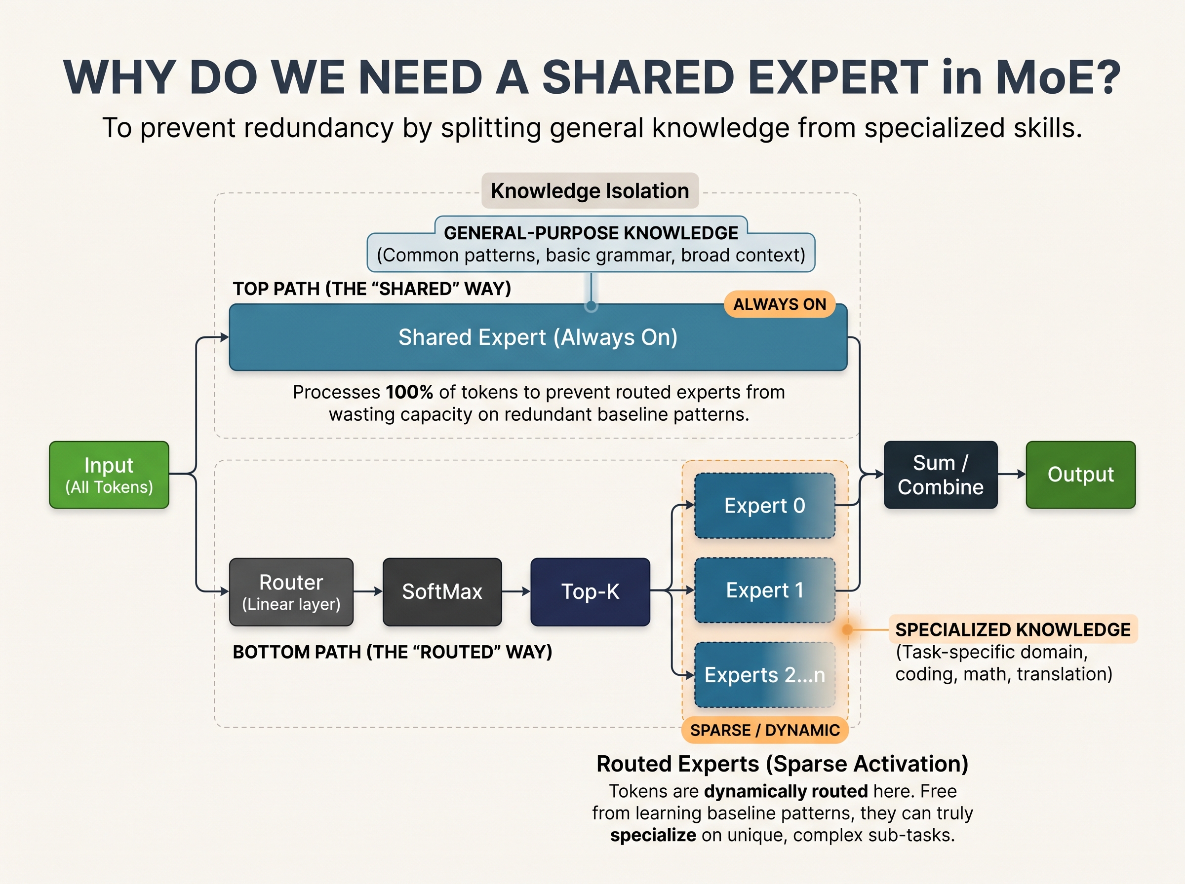
- Shared experts: process all tokens and play a role of the foundation which hold the general knowledge for all specialized experts.
6. References
| [^10]: [Stanford CME295 Transformers & LLMs | Autumn 2026 course](https://cme295.stanford.edu/syllabus/) |
-
Su et al., 2024. RoFormer: Enhanced Transformer with Rotary Position Embedding ↩
-
LLM Visualization - For inference but highly recommend to check ↩ ↩2
-
Devlin et al., 2019. BERT: Pre-training of Deep Bidirectional Transformers for Language Understanding ↩
-
Liu et al., 2019. RoBERTa: A Robustly Optimized BERT Pretraining Approach ↩
-
LLM Architecture Refresh: Inside a Transformer Block — Attention, Heads, and the FFN ↩ ↩2 ↩3
-
StackExchange: Why are residual connections needed in transformer architectures? ↩
-
He et al., 2016. Identity Mappings in Deep Residual Networks ↩
-
Dong et al., 2021. Attention Is Not All You Need: Pure Attention Loses Rank Doubly Exponentially with Depth ↩
-
Xiong et al., 2020. On Layer Normalization in the Transformer Architecture ↩
-
Fedus et al., 2022. Switch Transformers: Scaling to Trillion Parameter Models with Simple and Efficient Sparsity ↩