You can read more about GAN and special layers (i.e., up/downsampling, transposed layers) in CNN in this link.
Table of contents
-
What is Maximum Likelihood Estimation?
1.1. The Main Idea
1.2. Diffusion Process
1.3. Model Architecture
-
2.1. The Main Idea
2.2. Diffusion Process
2.3. Model Architecture
1. What is Maximum Likelihood Estimation? [4]
1.1. The Main Idea
In AI, we assume to have a set of parameters $\theta$ of a statistical machine learning model. And, our objective is to optimize our model parameters (denoted as $\theta$) to best fit the input data This process is called parameter estimation.
Maximum Likelihood Estimation (MLE) is one of 2 ways of parameter estimation. The estimation is conducted using only the training data.
| - Definition: The joint probability of $p(x_1, x_2,…,x_N | \theta)$ is called likelihood where $x_1, x_2,…,x_N$ are input data and we know their distribution represented the model $\theta$. Maximum likelihood is to find $\theta$ to maximize the joint probability, as shown as follows |
- Independence Assumption: It is difficult to solve (1), we need to assume that data points $x_N$ are independent. Therefore, we can approximate (1) by the below equation (based on Bayes’s rule and properties of independent variables)
\[p(x_1, x_2,...,x_N| \theta) \approx \prod_{i=1}^{N} p(x_i | \theta).\;\;\;\;\; (2)\]Then, our optimization problem is transferred into
\[\theta = \max_{\theta}{\prod_{i=1}^{N} p(x_i | \theta)}.\;\;\;\;\; (3)\]Also, optimization of a product is more challenging than that of a summation, then we will turn (3) into Maximum log-likelihood
\[\theta = \max_{\theta}{\sum_{i=1}^{N} log(p(x_i | \theta))}.\;\;\;\;\; (3)\]NOTE: MLE specifies the objective function, while optimization algorithms (e.g., Stochastic Gradient Descent) is a method to find the optimal solution for our objective function.
2. What is Diffusion Model? [1-3]
2.1. The Main Idea
Problems with existing models
GANs, VAEs, and Flow-based models shown their success in generating high-quality images. However, there are some limitations with them hindering their wide applications:
- VAEs: hinges on the surrogate loss.
- GANs: training instability and less diverse image generation problems.
- Flow-based models: relies on specialized architectures for reversible transform construction.
Solution: Diffusion (Probabilistic) Models (DPM)
Definition
- Diffusion probabilistic model: is a class of Generative AI and is a continuous time Markov stochastic process (a collection of random variables). It can generate high-resolution images with great accuracy in comparison with VAEs or GANs. For example, a Markov process can written as
\[P(X_{t_n}|X_{t_{n-1}},...,X_{t_{0}}) = P(X_{t_n}|X_{t_{n-1}}) \text{ with } t_0 < t_1 <...<t_n.\]Notebook for learning diffusion models using Diffusers
- We have a form for any diffusion process:
\[dX_t = a(X_t,t)dt + \sigma(X_t,t)dW_t.\]where $a$ is called the drift coefficient, $\sigma$ is called the diffusion coefficient and $W$ is the Wiener process. It is important to note that Wiener process make the equation stochastic.
2. Diffusion Process [3] - Must Read
Here are working flow of diffusion models via 2 processes:
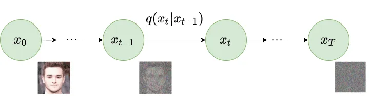
- Forward Diffusion Process (FDP): Input data is combined with Gaussian noise iteratively (i.e., Markov Chain) and randomly. In other words, we try to destroy the structure of input data’s distribution. The FDP progressively turn meaningful images (i.e., a complex data distribution) into a simple distribution (e.g., Gaussian noise) by adding noise. Here is a step of FDP:
\[q(x_t|x_{x_{t-1}}) = N(x_t, \sqrt{1-\beta_t}x_{t-1}, \beta_t I),\]where $q$ is the forward process, $x_t$ is the output of the forward process at time step $t$ given by input $x_{t-1}$, $N$ is a normal distribution, $\sqrt{1-\beta_t}x_{t-1}$ is mean, and $\beta_t I$ is variance. Especially, $\beta_t$ is often called schedule and ranged from 0 to 1.
NOTE: Schedule $\beta$ plays important roles such as scaling noise to be subtracted from the input int RDP.
Observation: The training process doesn’t use examples in line with the forward process but rather it uses samples from arbitrary time step $t$. Also, from the formula, we can see that at each training step, we need to iterate through $t$ steps (i.e., $x_t$ relies on $x_{t-1}$) to generate 1 data sample.
Solution: to make the FDP faster when we can calculate noise at any arbitrary time step $t$, where reparameterization trick $N(\mu, \sigma^2)= \mu + \sigma*\epsilon$ is applied to make the closed-formed computable (i.e., calculate $\overline{\alpha}_t$). Here is the entire FDP:
\[q(x_t|x_{0}) = N(x_t, \sqrt{\overline{\alpha}_t}x_{0}, (1- \overline{\alpha}_t) I) = \sqrt{\overline{\alpha}_t}x_{0} + \sqrt{1-\overline{\alpha}_t} \epsilon,\]where $\alpha = 1 - \beta_t$, $\overline{\alpha} := \prod_{s=1}^{t} \alpha_s$, and $\epsilon \in N(0,1)$.
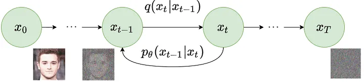
- Reverse Diffusion Process (RDP): Then, the model learns from the training process to remove these noises in this process or restore structure in data.
NOTE: Diffusion model (e.g., using neural networks) predicts the entire noise to be removed in a given time step. This means that if we have time step $t=200$ then our Diffusion model tries to predict the entire noise on which removal we should get to $t=0$, not $t=199$. Additionally, RDP consists of multiple steps in which a small amount of noise is removed at every step.
2.2. Unconditional/Conditional Generative Processes
- Unconditional Generative Process:
- Conditional Generative Process: In each decoder, we have attached text to have specific output.
3. Model Architecture
There are two common backbone architecture choices for diffusion models: U-Net (we can replace Resnet blocks with Attention Blocks) and Transformer.
4. Stable Diffusion
2.1. The main idea
Problems with Diffusion Models
The process of denoising is very slow and consumes a lot of memory when generating high-resolution images. Therefore, it is challenging to train these models and also use them for inference [5].
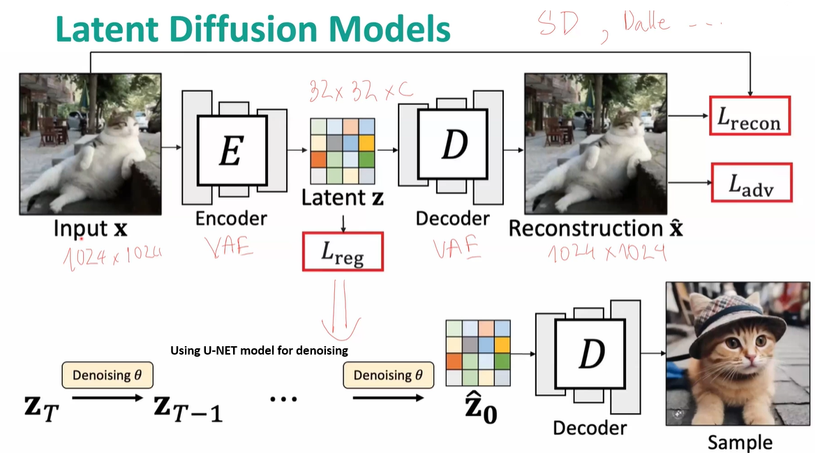
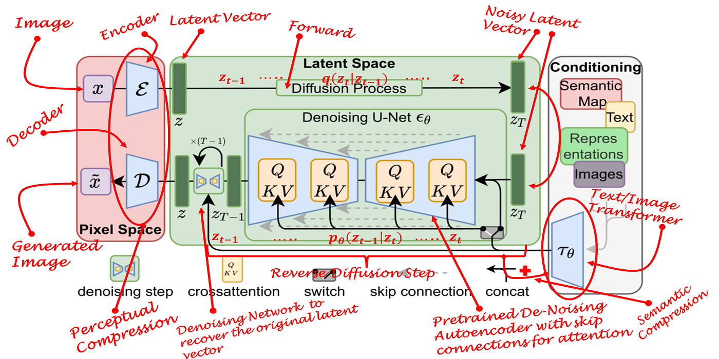
Solution: Latent diffusion can reduce calculation costs (e.g., time and computation complexities) by creating a latent representation over a lower dimensional space, instead of using the actual pixel space.
- Stable diffusion is based on Latent Diffusion Model. Particularly, they encode text inputs into latent vectors using pre-trained language models like CLIP.
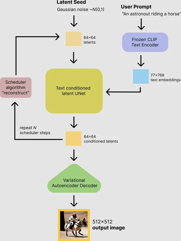
2.2. Main components
Variational Autoencoder (VAE)
The image input will be compressed into a low dimensional latent space, called noisy latents, by using encoder. Then, this encoded latent will be fed into U-NET model. At the end, for inferencing, we use decoder to convert denoised image into actual image.
U-NET model
We can predict the added noise in the noisy latent using U-NET. By doing so, we can get the actual latents by subtracting the noise from the noisy latent.
Text-encoder, e.g., CLIP
Text prompts will be converted into an embedding space using the pre-trained text encoder (e.g., CLIP), that will then be the input of U-NET.
Scheduler
Scheduler defines the whole de-noising process (e.g.,the number of de-noising steps, stochastic or deterministic steps, algorithms for de-noising). To know more about the differences between these kinds of schedulers, check this link [7].
5. NOTE
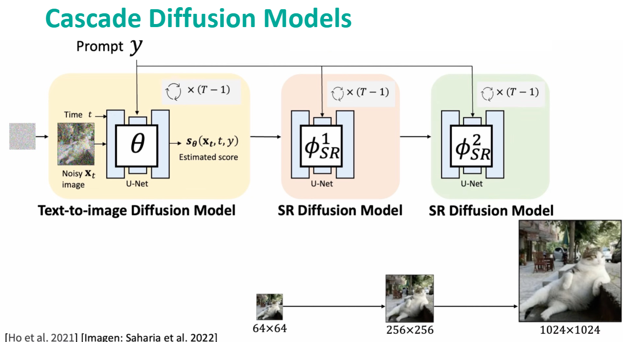
- How to generate big and high-resolution images?
**Answer**: In addition to Stable Diffusion models, we can use Cascade Diffusion Models.
- How to speed up the image generation process? For example, running time of Diffusion = (T-1) x Running time GAN/VAE.
**Answer**:
-
Denoising Diffusion Implicit Models (DDIM): It does not require $q(x_t x_{t-1})$ to be a Markov process. -
Progressive Distillation: It reduces the number of steps.
-
Guided Distillation: It combines Progressive Distillation and Latent Diffusion Models.
-
Consistency Models:
- Low-rank Adaptation (LoRA): civitai
6. Summary [6]
- Variational AutoEncoders (VAEs): The encoder encodes data towards a distribution close to a gaussian, or data is compressed into a lower-dimensional latent space, whereas the decoder reconstructs data from the latent space.
- GANs: A generative network G is trained to take a random input (from a gaussian, for example) and to output a data from the target distribution. A discriminative network D is trained to differentiate true data from generated data.
- Diffusion Probabilistic Models (DPMs): learn the reverse process of a well defined stochastic process that progressively destroy information, taking data from our complex target distribution and bringing them to a simple gaussian distribution. Specifically, it takes gaussian noise as an input and generating data from the distribution of interest.
Reference
1. A Very Short Introduction to Diffusion Models
3. Step by Step visual introduction to Diffusion Models.